Occupancy estimation and forecasting for energy savings

Written by Clement Cruveiller – SEM 3A ENSE3

ABSTRACT

With the new climate incentives European countries are looking for carbon neutrality in 2050. The building sector is responsible for almost 40% of the primary energy consumption. If building renovation and using energy efficient systems, the IEA in Annex 66 relates that the energy efficient efforts can not go without a behavioural change from the occupants. Optimistically occupants can become more and more sober in their energy consumption, but the transition will not be that easy. The goal of this miniproject is to create an interactive application based on a predictive controller that enables energy savings but also awareness raising for occupants. The predictive controller needs to be able to forecast the occupancy based on machine learning techniques. The study is based on the Smart ExpHouse platform of Grenoble laboratory G2eLab.

Introduction

In order to create a predictive controller we need to acquire many data related to the occupant behaviour in the building, consumption, co2 concentration, humidity, temperature etc… For this many sensors need to be installed in order to acquire this data and then analysed to get the desired information. First part of this paper will present the data acquisition, the second part how to estimate the occupancy from the measured data, third part tackles how a prediction could be made form this data and finally an approach to save energy will be discussed.

Smart ExpHouse

The SmartExp house is a residential house of two floors with many sensors.

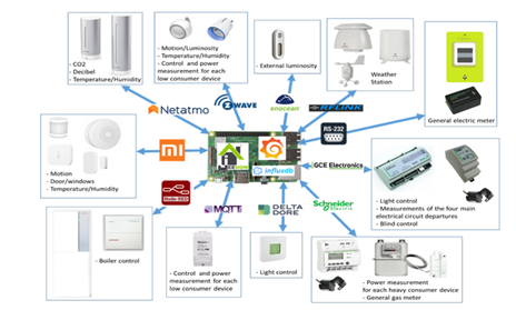
Figure 1: Smart ExpHouse architecture

There are different sensors connected to the different wireless networks and all the data is available on Grafana thanks to InfluxDB that created the datasets. The servor used is on Jeedom and we is connected to the different measures thanks to different wireless communication devices like Enocean.

From the Grafana we used different measures exported to csv in order to use them on python.

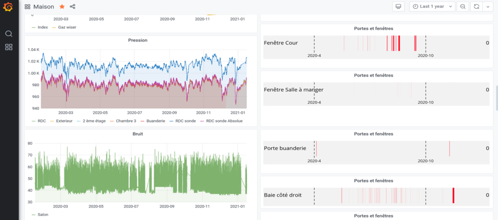
Figure 2: Grafana Data Visualisation

Occupancy estimation

It is a hot topic these last years to measure or estimate the occupancy mostly thanks to data related to CO2, acoustic pressure, power consumption and other. Unfortunately, most of this techniques are depending on supervised machine learning techniques meaning that for one input of CO2, acoustic pressure and power consumption we obtained through an intrusive technique like cameras the associated occupancy. In our case we don’t have access to the real occupancy so we are going to use machine learning unsupervised methods.

Since it is difficult to estimate with accuracy the number of people in the room, I have decided to detect the occupancy in the house. For each clustering we are having a look into the silhouette which is an indicator of the quality of the clusters, the closer we are to 1 the better our clusters are defined.

We first use the CO2 in the house, the power consumption and the noise:

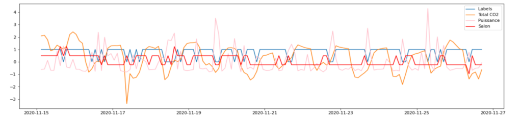
Figure 3: Clusters plotted with power, co2 and noise

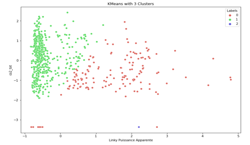
Figure 4: Clusters with power, co2 and noise

Silhouette: 0.467

With this approach it looks difficult to estimate the occupancy since we don’t have clear clusters that are more created according to the power consumption than the other parameters. The bad quality and simplicity of the clusters can be explained by noise data that doesn’t give a lot of information ince there is always noise in the house which could be do to the cars.

In the next approach we are using only the total cO2 level in the house and the total power consumption. We can clearly see that the pattern detected by the clustering makes sense with a pattern that could have been related to the occupancy, indeed we can see below that there is on the left corner a cluster corresponding to low power consumption and low CO2 that probably coincides with absence in the house, the purple one should represent the sleeping time in the house and the green one the day, this clustering even if there is no scientific way to confirm these results seem to make a good estimation.

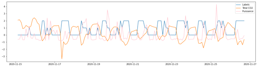
Figure 5: Clusters plotted with power, co2

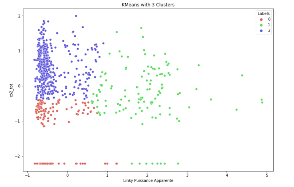
Figure 5: Clusters with power and co2

Silhouette = 0.480

By curiosity I then tried to increase the number of clusters to confirm that the “absence” cluster would not split into two new clusters, hopefully as we can see below this not happened, we got the top left corner that split into two new clusters. This experiment confirms that the 3 clusters above can make a correct estimation of the presence in the house.

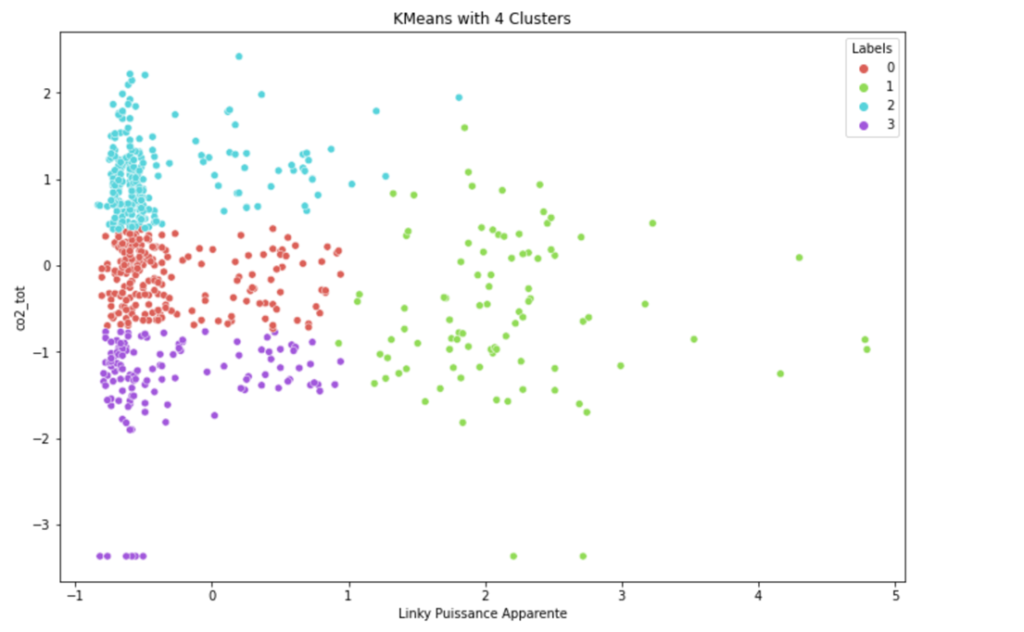
Figure 6: Introducing one additional cluster

Silhouette 0.40

Occupancy forecasting

Now that we have created a model to detect the occupancy we can work on a model that would be able to forecast the occupancy, for this we could use a simple regression model. The occupancy in this model is built only according to past data. To implement a forecasting model I have implemented a MLP model that I had already studied in ICT course. When we have a look into the forecasting techniques most people praise the fact that it is not really the model that you use that will give you great accurate model but rather the way you handle the available data. In order to create a suitable dataset for the model some feature engineering must be done.

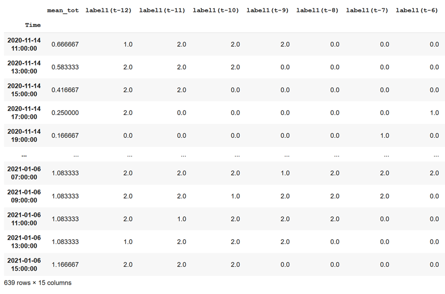
Figure 7: Feature engineering

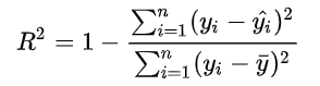
As you can see in the picture above, the occupancy dataset is converted into a multiple columns dataset wich includes the past data you want to use to predict the next desired steps of occupancy, for example here I decided to forecast 4 hours ahead using the last day. In order to train the model I have used 70% of the dataset and 30% for the testing. The following R2 Score I obtained, which is expressed as below (the closer to one the better the model).

Always supposing occupancy=1	-0.024
4 hours forecast using 2 days past data	0.15
4hours forecast using 1 day past data	0.32
4 hours forecast using 1.5 day past data	0.22
4 hours using 20 hours past data	0.25
4 hours using 1 day past data introducing mean as feature	0.38

Table 1: Forecasting Results

The first test was basically to get a starting point which we could start with to see if the model was heading the good direction. Unfortunately 24 hours forecasting results were really poor so I have chosen to work with 4 hours, the objective of the model is to predict presence or absence in the house.

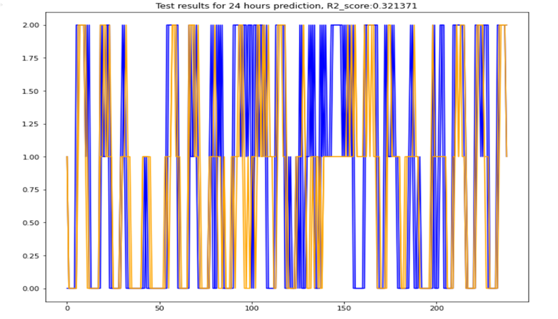
Figure 8: 4 hours prediction with 1 day past data

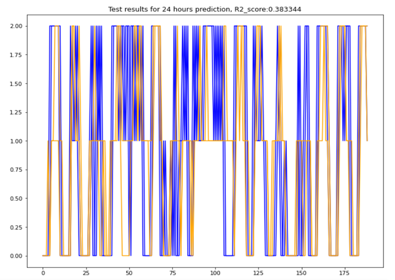
Figure 9: 4 hours prediction with 1 day past data + mean feature

The results are not really accurate we are not even going beyond 50% of r2 score, yet we managed with simple data manipulation to almost double the R2 score. With hypertuning (which I did manually) and more data features analysis probably good result could be achieved (for a data scientist it would have been 0.8 at least).

Energy savings

Finally the idea is to put into application our forecasting model to make some energy savings. For this we need to need the thermal behaviour of the house. For example, how does the average temperature is changing according to the known parameters and also how much heating power do we need to be at a certain comfort temperature. To do that rather than using model from physics knowledge we could use the observed behaviour of the house using some simple machine learning regression.

 For example, let’s study the temperature, since there are a lot of rooms the simulation could be complicated. I have tried for example with the indoor average temperature for example. Let’s try to make a regression model using a multi-input and multi-output using the features of: outdoor luminosity, power consumption, estimated occupancy at step t and t-1. Unfortunately it needed quite some data modification to take into account the gas heating power, since the time samples was randomly introduces, that could have strongly improved the model. The results obtained in a reasonable amount of work time weren’t great so I have decided not to go further in this part.

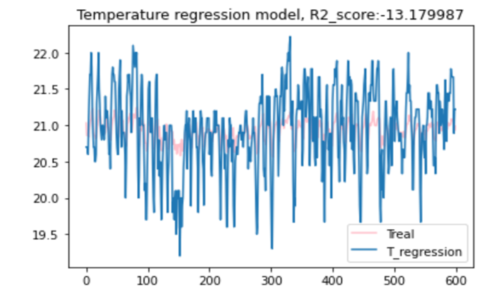
Yet from a simpler one room office in another project studying the GSCOP office in Grenoble I was able to reproduce a correct model for temperature since there was less parameters to take into account.

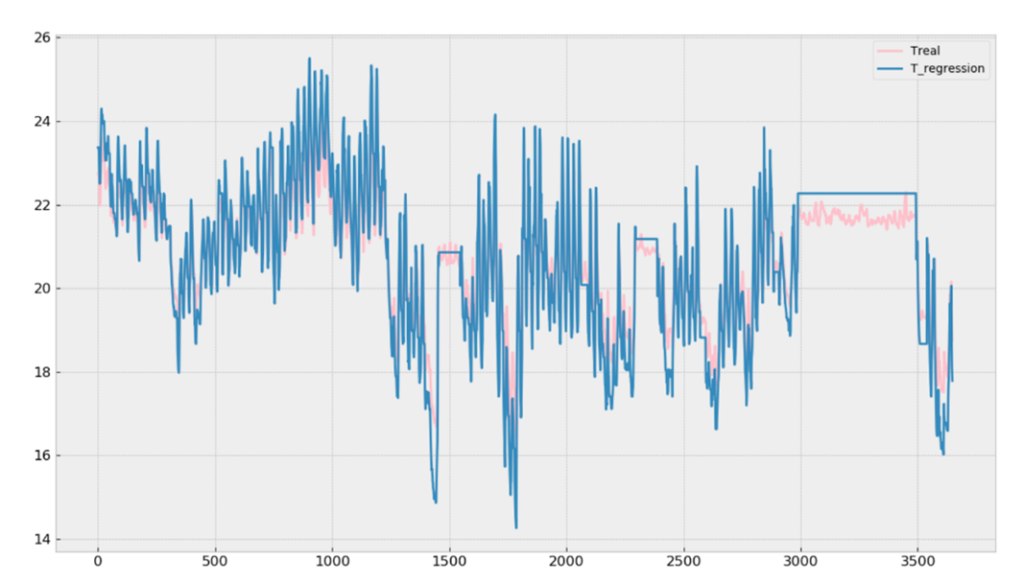
Such a regression implemented for the temperature the CO2 level, and the input heating power enabled to model on python a real simple predictive controller that worked as explained below that could be connected to a boiler through a Raspberry Pi

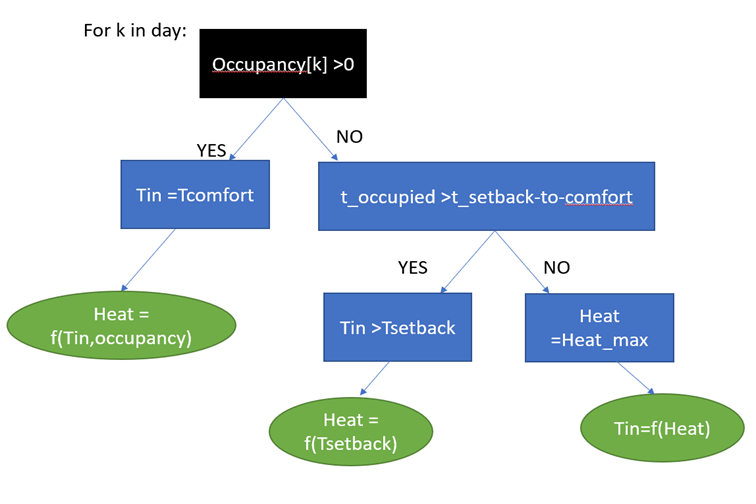
Figure 10: Controller architecture

Below you can see the resulting heating power input in the small office that resulted in more than 50% of energy savings of course the simulation is not very realistic but it seems to be a promising technique.

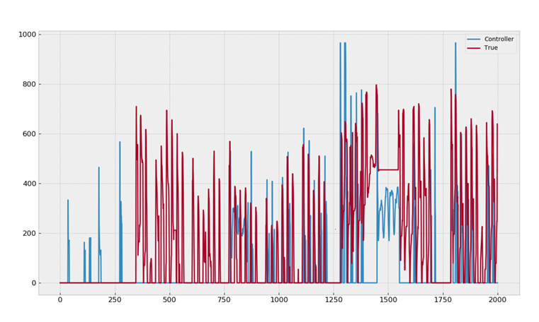
Figure 11: Energy savings Controller vs True

Conclusion

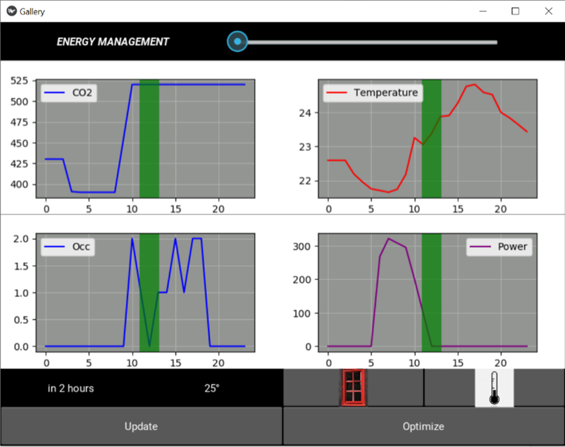
Implementing sensors in a house can give a lot of information on the daily behaviour of the occupants. In my house I am lacking information to perform a good model for example a true observation on the number of occupants, data related to the occupants calendar or even GPS information… There are a lot of interesting insights that I could have focused on more as for example studying individually each room to have a less general approach.  But energy efficient homes can be built but the engineer can’t do a lot regarding the occupants behaviour. Implementing a few sensors during a few months to study the energy dynamics of the house presents a lot of way to raise awareness regarding potential energy savings. For example CO2 level in the house can detect occupancy, observing th occupancy during a few days could help building a predictive a model with python libraries that are becoming more and more easy to use. This predictive model thanks to a building model that could be built with data observations could through a daily planned energy strategy result in considerable energy savings by implementing a Raspberry Pi that costs no more than 30 euros. Finally all this ICT technology should be a way to influence people towards efficient energy behaviours for example with the help of an interactive App that would tell the occupant when is the best time to open the window, or to correct its occupancy prediction. Below is an example of a Kivy UI very simple app I have implemented that is a GUI that works with Raspberry Pi.

Bibliography

EXPE-SMARTHOUSE – The Full Connected Living House. http://expe-smarthouse.duckdns.org/?page_id=7&lang=en. Consulté le 17 janvier 2021.

Mishra, Sanatan. « Unsupervised Learning and Data Clustering ». Medium, 21 mai 2017, https://towardsdatascience.com/unsupervised-learning-and-data-clustering-eeecb78b422a.

Manar Amayri, Stéphane Ploix, Sanghamitra Bandyopadhyay. Estimating Occupancy in an Office Setting. The First International Symposium on Sustainable Human-Building Ecosystems (ISSHBE)